Showing posts with label Ms Excel. Show all posts

Saturday, May 17, 2008

Memasukkan Baris atau Kolom dengan Keyboard

Memasukkan Baris atau Kolom Baru - dng Keyboard

Insert a New Row or Column - Excel Keyboard Shortcut

Untuk memasukkan baris atau kolom baru dengan keyboard, tanpa mouse maka dua langkah dibawah ini dapat diterapkan
  1. Shift+SpaceBar = Pilih baris (row)
  2. Ctrl+Shift+PlusSign = Insert Baris (row)
Sedangkan untuk column, maka langkah pertama adalah Ctrl+SpaceBar untuk memilih kolom. Untuk memasukkan lebih dari satu baris atau kolom maka gunakan tombol panah keyboard bersama-sama tombol Shift sebelum melanjutkan ke langkah ke dua.

Sunday, May 11, 2008

Menggunakan Tabel Pivot untuk Meringkas Data

Misalnya anda memiliki data penjualan yang isinya 50.000 baris seperti terlihat pada Gambar 1

Dengan data itu anda ingin membuat laporan ringkas yang menunjukkan penjualan per wilayah dan produk (region and product).

Gambar 1. Ringkas tabel data berikut.


Caranya: Untuk
meringkas data di atas, anda dapat menggunakan pivot table. Pivot tables sngat cocok untuk analisis data seperti di atas.

Peringatan: Pivot tables di Excel 2007 sangat berubah dari versi

Excel 97-2003. Untuk membuat ringkasan pendapatan berdasarkan wilayah dan produk membutuhkan klik mouse sebanyak 4 kali dan satu kali tahan tarik mouse (drag):

Pastikan bahwa data yang ada dalam daftar memiliki judul (pada baris paling atas) yang berbeda satu dengan lainnya (unik).

Pilih salah satu sel dalam database (data anda). Pilih Menu Insert – Pivot Table.

IntelliSense Excel (sensor cerdas Excel) akan menduga range data anda. Dan biasanya benar seperti pada Gambar 2. Dan Klik OK.


Dengan menekan tombok OK, anda akan melihat tabel pivot yang masih kosong dan dua toolbar tabel pivot baru, dan sebuah dialog daftar PivotTable baru. Dialog Excel versi 2007 memperlihatkan daftar filed pada bagian atas dan empat tempat meletakkan (Drop Zone) field pada bagian bawah dialog, seperti terlihat pada Gambar

Sedangkan pada Excel versi sebelumnya, maka anda harus menarik field dari Dialog Field

List langsung ke pivot table. Proses ini sangat menyulitkan bagi orang yang masih baru mengenal pivot tables. Dalam Excel 2007, anda menarik field dari dialog field list bagian atas ke zona yang yang cocok pada bagian bawah dialog Field List. Biasanya dengan hanya meng-klik field yang ada di dialog Field List akan menempatkan field tersebut pada zona yang tepat. Untuk kasus yang kita miliki ini, maka kita mencoba meletakkan produk merupakan daftar yang ke bawah (judul baris) sedangkan wilayah merupakan judul mendatar (judul kolom).


Gambar 3. Dialog PivotTable Field List di bagian atas dan Drop Zone di Bagian Bawah


Klik Check box Produk di Dialog Field List bagian atas. Excel akan secara otomatis memasukkan ke dalam Row Labels (Label baris) pada drop zone. Pivot table akan menunjukkan daftar produk satu per satu (tidak ada duplikasi) pada Kolom A (lihat Gambar 4).


Gambar 4. Klik sebuah field text, dan Excel memasukkan field itu ke area Baris.


Klik check box Pendapatan yang ada di dialog Field List bagian atas. Dan karena field tersebut adalah numeric maka Excel akan menambahkan pada bagian Values (nilai) dari pivot table.

Jika anda meng-klik check box Wilayah, maka Excel akan meletakkan field tersebut di area row pada pivot table. Karena anda ingin wilayah menjadi judul kolom maka, klik mouse, tahan dan tariklah field Wilayah dari dialog Field List dan letakkan di drop zone Column Labels yang terletak di bagian bawah dialog Field List.

Hasilnya adalah ringkasan data penjualan berdasarkan produk dan wilayah, seperti terlihat dalam Gambar 5.


Gambar 5. Pivot table membuat anda mudah untuk meringkas laporan.


Tingkat Lanjut: Pivot table memberikan banyak opsi (pilihan) yang sangat berguna. Untuk mempelajari lebih lanjut klik disini

Untuk Pemakai Versi Sebelumnya: Jika anda menyukai pivot table pro pada Excel versi sebelumnya, maka anda akan dengan cepat menggunakan pivot table

Excel 2007. Drop zones telah diubah namanya. Drop Zone Row Area sekarang bernama Row Labels. Sedangkan drop zone Column Area sekarang menjadi Column Labels. Drop Page Field menjadi Report Filter. Dan drop zone Data Area menjadi Σ Values (walaupun saya menyebutnya drop zone Values, dengan mengabaikan symbol Σ).

Agar Lebih Mudah: Pada
awal pembuatan sebuah Pivot Table, maka dialog PivotTable Field List akan berada di layar sebelah kanan. Anda dapat memindahkan ke tengah dengan cara klik pada Judul Dialog dan tarik ke worksheet agar terlihat mengambang di atas worksheet dan mempermudah anda dalam mengatur data. Dalam membuat artikel ini saya menggeser ke tengah agar tampak dalam gambar yang disajikan sebagai contoh.

Bentuk Drop Zone: Anda dapat mengatur bentuk dialog PivotTable Field List dengan mengklik dropdown pada bagian atas. Bentuk yang ditawarkan untuk tampilan ini ada lima (5). Tiga diantaranya tidak menyertakan daftar field atau drop zones. Jika tampilan dialog box anda tidak menampilkan salah satu bagian tersebut, maka gunakan panah dropdown untuk mengembalikan tampilan ke Fields Section and Areas Section Stacked. Ada juga yang menampilkan field dan drop zone secara berdampingan.

Kesimpulan: Perintah
Insert – Pivot Table dapat meringkas ribuan baris data secara cepat. Excel tidak membutuhkan anda mengerti rumusnya. Anda hanya harus dapat meletakkan field ke dala tata letak (layout) laporan.

Perintah Di Menu: Insert – Pivot Table

Wednesday, May 7, 2008

Mengecek Umur Dalam Excel

Misalnya kita punya daftar tanggal lahir beberapa orang, kemudian kita mau mengecek yang berumur 18 tahun ke atas maka dalam excel kita dapat menghitung sbb:

Untuk mementukan apakah umurnya 18 tahun atau lebih ( hasil TRUE berarti benar)

Rumus di Kolom Cek umur

=AND(ISNUMBER(A1),(A1-1)< style="font-weight: bold;">

Kolom Dikembangkan


=IF(AND(ISNUMBER(A2),(A2-1)< style="font-weight: bold;">Hasilnya
Tgl Lahir Cek umur Dikembangkan
4/19/1962 TRUE Ya tuh sudah tua
4/20/1992 FALSE Masih muda koq


Menghitung Umur dalam Excel

Untuk menghitung umur dalam Excel


Fungsi yang dapat digunakan untuk menghitung umur dalam excel adalah DATEDIF

Penggunaannya adalah sebagai berikut:

=DATEDIF(A1,TODAY(),"y")
atau
=DATEDIF(A1,NOW(),"y")


Sebagai alternatif dengan menggunakan rumus yang agak panjang adalah

=TEXT(IF(OR(MONTH(TODAY())>MONTH(A1),AND(MONTH(TODAY())=MONTH(A1),
DAY(TODAY())>=DAY(A1))),(TODAY()-A1)/365.25,(TODAY()-A1)/365.25-1),"0")


Tinggal pilih yang mana ... mau panjang dan lama atau cepat ... Kalau untuk jarak tanggal ya Today() atau Now() diganti tanggal aja

Ini adalah iklan :

Search internet dapat uang

Clicks - data Uang

Pamer Diri dapat Uang

Rumus Array (CSE) dalam Excel

Rumus Array berbeda dengan rumus biasa yang kita masukkan dalam excel. untuk memasukkan rumus ini kita perlu dua hal berikut

1. Pada saat memasukkan rumus untuk array, maka pertama pilih range (ingat range bukan sel) yang akan diberi rumus, kemudian masukkan rumusnya, setelah selesai tekan Ctrl, Shift dan Enter setaca bersamaan (jangan hanya tekan Enter saja)

2. Pada saat kita memasukkan rumus array, maka akan muncul dua kurung kurawal seperti pada contoh di bawah ini

{=Rumus Yang Kita Masukkan}

Dan Yang Perlu Diingat ::::: Jangan memasukkan kurung kurawal sendiri dengan mengetikkannya, Excel akan otomatis membuat kurung tersebut dengan kita menekan CSE (Ctrl, Shift dan Enter)

Friday, February 29, 2008

Menghitung NPV, IRR, xNPV dan xIRR dng Excel

Menghitung NPV, IRR, xNPV dan xIRR dng Ms Excel

  1. NPV (Net Present Value)
    NPV adalah selisih antara present value dari investasi dengan nilai sekarang dari penerimaan-penerimaan kas bersih di masa yang akan datang. Untuk menghitung nilai sekarang perlu ditentukan tingkat bunga yang relevan.
  2. IRR (Internal Rate of Return)
    Metode IRR ini digunakan untuk mencari tingkat bunga yang menyamakan nilai sekarang
    dari arus kas yang diharapkan di masa datang, atau penerimaan kas, dengan mengeluarkan investasi awal. Caranya, dengan menghitung nilai sekarang dari arus kas
    suatu investasi dengan menggunakan suku bunga yang wajar, misalnya 10 %. kemudian
    di bandingkan dengan biaya investasi, jika nilai investasi lebih kecil, maka di coba lagi
    dengan penghitungan suku bunga yang lebih tinggi demikian seterusnya sampai biaya
    investasi menjadi sama besar. Apabila dengan suku bunga wajar tadi nilai investasi lebih
    besar, maka harus di coba lagi dengan suku bunga yang lebih rendah sampai
    mendapatkan nilai investasi yang sama besar dengan nilai sekarang.
File Excel contoh perhitungan dapat di download disini

Some NPV resources

Tuesday, February 19, 2008

Excel 2003 Tutorials from Kansas University

Here are 4 illustrated Excel 2003 Tutorials from Kansas University that demonstrate how use use many important features of Excel. These tutorials take you step-by-step through each task being taught using screen shots and easy-to-follow instructions.

Excel Introduction Tutorial

This introductory Excel tutorial will get you going with using Excel to perform fundamental tasks, such as creating, saving, and opening new Excel workbooks and worksheets; selecting, copying, and moving data; constructing formulas; formatting worksheets; and setting up worksheets for printing. (22 pages, 424kb, pdf format)

After using this Excel tutorial, you will be able to:
- Create, open, and save Excel workbooks
- Select, copy, and move data
- Create formulas using relative and absolute references
- Format worksheets
- Use Page Setup to set up worksheets for printing

Contents of Excel Introduction Tutorial:
Introduction
Objectives
Definitions
Creating and Opening Excel Workbooks
Inside an Excel Worksheet
Creating Formulas
Editing & Deleting Formulas
Copying Formulas and Values
Changing the Workbook or Worksheet Appearance
Getting Additional Help


Excel Data Management Tutorial
This Excel 2003 tutorial describes you how to use Excel to work with lists, data forms, filtering, and subtotals features, along with managing windows and link to data and formulas. (18 pages, 267kb, pdf format)

After using this Excel tutorial, you should be able to:
- Sort a data list
- Filter a data list according to criteria
- Extract data list information
- Use the subtotal function
- Adjust the spreadsheet windows

Contents of Excel Data Management Tutorial:
Introduction
Objectives
Using Excel lists
Creating a List
Sorting
To perform a Simple Sort
To Sort by Multiple Columns
Data Forms
Adding Data Using the Data Form
Finding Records Using Criteria
Filtering Data
AutoFilter
Advanced Filters
Special Features for Filtered Lists
Totals and Subtotals
Total Row
Subtotals
Managing Windows
Multiple Windows
Splitting Windows
Freezing Panes
Linking Data
Getting Additional Help


Excel Tutorial on Functions and Data Analysis Tools

This Excel 2003 tutorial will show you how to use Excel's functions and data analysis tools. Topics explained include functions such as Average and Sum, and data analysis tools such as pivot tables and conditional summations. (19 pages, 371kb, pdf format)

After reading and applying this Excel tutorial, you will be able to:
- Define terms related to using functions
- Create and edit a function
- Identify add-in functions
- Perform data analysis using Data Analysis Tools
- Create a formula with the Conditional Sum wizard
- Learn to troubleshoot a formula

Contents of Excel Tutorial on Functions and Data Analysis Tools:
Introduction
Objectives
Definitions
Inserting Functions
Sample Functions
Add-In Commands and Functions
Loading an Add-In
Unloading an Add-In
Data Analysis Tools
Histogram
Conditional Sum
Analyzing Data with the PivotTable
Array Formulas
Getting Additional Help


Excel Charting Tutorial

Learn how to use Excel to create and edit charts, modify chart options, and format chart objects, as well as use trendlines, forecasts, and error bars to present data graphically. (17 pages, 361kb, pdf format)

You will be able to do the following after going through this Excel tutorial:
- Create and edit charts
- Modify chart options
- Format chart objects
- Apply trendlines and error bars

Contents of Excel Charting Tutorial:
Introduction
Objectives
Definitions
Creating a Chart
Using the Chart Wizard
Modifying Charts
Formatting Chart Objects
Trendlines
Pie Charts
Creating a Pie Chart
Printing Charts
Printing an Embedded Chart on a Separate Page
Getting Additional Help

Microsoft Excel Ti[ps and Tricks


Microsoft Excel Tip Categories

Please select a category from the list below:

Excel General
Excel General
Excel Text, Editing and Format
Excel Date and Time
Excel Date and Time
Excel Formula and Function
Excel Data
Excel Data
Excel Macros and VBA


Excel General Excel Text, Editing and Format Excel Date and Time Excel Formula and Function Excel Data Excel Macros and VBA

Sunday, February 10, 2008

Ms Excel - Formatting Entries

Formatting

Formatting is anything that changes the appearance of an entry: alignment, number of decimals used to display a number, font typeface, font style (bold, italic, or underlined), font size, font colour, borders around the cell, a coloured background for the cell, etc. In addition, we may change the width of a column and the height of a row, and text may be centred over a number of cells. You may format cells one-by-one or, by first selecting a number of cells, all the cells in a range may be formatted at one time.

Clearly the Formatting toolbar provides many tools to change the appearance of a cell. If you let the pointer linger over a tool icon, a tooltip will appear telling you the purpose of the tool. You should use this method to identify the tools to change the font typeface, size and style (bold, italic and underlined). In the same way, find the three tools to change alignment.

Each of the tools which add borders, change the font colour and add a coloured background (pattern), has a small V beside it to indicate that the tool leads to a dialog box. Note that the border tool provides only black borders, below we see how to get coloured ones. Recall that the tools are a subset of the menu commands.

Other tools on the Formatting toolbar may be used to change how numeric values are displayed. Locate the Increase decimals and the Decrease decimals tool, and the tools to change the display to currency, as a value with thousand separators, or as a percentage.

6 Getting Started with Excel

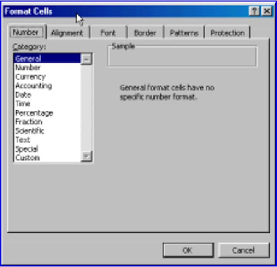
The menu command Format|Cells opens up the dialog box shown in Figure 6. From the Number tab one can set the format for numbers. The default setting is called General. You may wish to experiment with the Fixed and the Currency setting. If you click on the Fraction item you will see that it is possible to have fractional values displayed as quarters, eighths, etc.

Figure 6

The command Format|Column may be used to alter the width of a column. The default width is 8.38 units. A group of columns may be altered by selecting them in the column heading row before opening the Format|Column dialog. One of the most useful items on this dialog is the AutoFit Selection which makes the columns just the right width to hold their contents. If a column is given a width that is too small to hold a numeric value, the value will be displayed as ########. The solution is to (a) widen the cell and/or (b) display the value with fewer decimals if possible.

To experiment with formatting, make the worksheet shown in Figure 7. The vertical text was typed in normally and the cells were formatted with Format|Cells and opening the Alignment tab. The columns with this text were formatted for AutoFit. Using Tools|Options, and opening the View tab, the gridlines were removed from this worksheet.

Training completed

Cash register

Customer inquiry

Inventory check

Damian

x

x

Jo

x

x

Justin

x

Nichola

x

x

Simon

x

x

Tim

x

x

x

Ms Excel - Cell References and Entries

Cell References

To refer to a specific cell we use a cell reference. This is a combination of the column heading and the row number. The cell at the top left, which is at the intersection of column A and row 1, has a cell address of A1. The cell below is A2 while the cell to the right is B1. This method of naming cells using the column letter is called the A1 method. To reference a cell on another sheet of the same workbook, we use the form Sheet2!B4 – note the exclamation mark. To reference a cell in another workbook we can use the form 'C:\My Documents\[Book2.xls]Sheet1'!$A$1. We discuss the dollar signs in a cell reference later in this chapter.

Cell Entries

A cell may contain data or a formula. A data entry may be: a number, text (sometimes called labels) or a date. Formulas begin with an equal sign (=). We discuss formulas in detail in the next unit.

You may wish to experiment by making the worksheet shown in Figure 4. Type the entries in cell A1, C1, G1 and in row 2. For example, with A1 as the active cell, type the word Text and press the R key to complete the entry. We will discuss other ways of completing a entry later. Click on C1 and enter the next piece of data.

A

B

C

D

E

F

G

1

Text

This is an example of a long text entry

123456789

2

123

1.5

1.55

1 1/2

1.23457E+14


Figure 4

A number of observations may be made about how entries are initially treated. Later we

will discuss how formatting may be used to change the appearance.

1) Text is left aligned by default. By this we mean that on a newly opened worksheet any text typed into a cell will be placed to the left within the cell. The alignment may be changed by formatting the cell.

2) By default, numbers are left aligned.

3) Text can overflow into empty adjacent cells as shown by the entry in C2. If you type anything in D2, only part of C2's entry will be visible in the cell but all of it will be visible in the Formula bar.

4) When a large number (not too large) is entered, the column automatically widens to accommodate all the digits.

5) Very large numbers (the value typed into G2 was 123456789123456) are converted to exponential (sometimes called scientific) notation. The displayed value 1.23457E+14 means the same as 1.234567 × 10¹⁴. In the next unit we discuss Excel’s precision.

6) A whole number can have no more with than 15 digits. You are unlikely to be working with numbers that large. Objects we often call numbers are really just a string of digits. For example, phone numbers and account numbers are not real numbers in that we never perform arithmetic operations on them. In these cases it is better to enter the value by first typing a single quote (it is found on the key next to R). This quote mark will not be displayed in the cell but will cause the entry to be treated as text.

7) By default, Excel does not display what it considers to be insignificant digits. Thus if you type 1.50 in B2, the value 1.5 will be displayed in the cell and in the formula bar. Again, formatting can be used to change this.

8) Fractions may be entered as in D2. Note there is a space between the 1 and the 1/2. If you wish to enter a fraction (for example, 1/2) without a whole number, you must enter it with a preceding 0 followed by a space (e.g. 0 1/2). The zero will not be displayed when the entry is completed. In all cases, the values displayed in the Formula bar will be in decimal form (e.g. 1.5, or 0.5).

9) To evaluate a number in fractional notations, enter it as a formula. Thus to display the result of 1½ + 3¾ enter = 1+1/2+3+3/4. See the next unit for more on formulas.

10) Improper fractions are converted on entry. Thus 1 4/8 will be converted to 1 1/2. In certain cases (when the denominator is 2, 4, 8, 16, 10 or 100) we may format the cell to overcome this.

11) If you enter something like 4/12 without a leading zero, Excel will take this to mean a date – either 4 December or 12 April depending on your Regional Setting. We will not be discussing dates in this supplement.

We indicated above that you need to let Excel know when you have finished entering something in a cell and recommended the use of the R key. This is not the only way. Any of the navigation keys (B, L , R , T) and T may be used. Alternatively, you may click the Tin the Formula bar – this is displayed only while a cell entry is being made or edited. Do not get into the bad habit of clicking the mouse on another cell to complete an entry. While this will work when you are entering data it will cause you grief when working with formulas.

Ms Excel - Toolbars

Toolbars

As with all Windows applications, the toolbars provide quick access to the more frequently used menu commands. That is to say, the commands available from toolbars are a subset of the menu commands. In Excel2000 the Standard and the Formatting toolbars are docked together on one row by default. This means that only part of each toolbar is visible. To see the hidden part, click on the double arrow. If you prefer to have the toolbars on separate rows, open the Customize dialog box as explained above and clear the check mark from the box labelled Standard and Formatting toolbars share one row.

The amount of space allocated to each toolbar when they share a row may be changed. With the mouse, click on the vertical bar to the right of the first double arrow and drag it to one side.


Microsoft Excel Menu Commands

Menu commands

The menus in Excel 2000 are similar to menus in other Windows applications. However, as with all the Microsoft Office 2000 products there is a small difference from earlier versions: when you open a menu item an abbreviated version is displayed (Figure 2.)

Figure 2

Getting Started with Excel 3


Figure 3

The menu shows the commonly used and the most recently used commands. The entire menu is displayed if you click on the down arrow at the bottom of the menu. If your version of Excel is so configured, the full menu will also appear after a short delay. To configure Excel, either use the command Tools|Customize or right click on the menu bar and select the Customize item. In either case, the Customize dialog box is opened. If you move to the Option tag, the dialog box resembles Figure 3. To have all the commands displayed, clear the check mark from the Menus show recently used commands first box. Beaware that this action will affect other Microsoft Office 2000 application on your PC.

Menu commands may be accessed by clicking on the required item. Alternatively, you may hold down the A key and press the key corresponding to the underscored letter in the menu item. Thus the File menu is opened with A+F. A third method is available for other commands. If you open the File menu you will see to the right of the Save item the shortcut CTRL+S. This means that the key commination C+S will save the current file – there is no need to open the File menu for this to work. The shortcuts for copy and paste (C+C and C+V) are very useful to know.

Student resources for Quantitative Approaches in Business Studies

Student resources
Excel supplement
The Excel supplement is a tutorial for Microsoft Excel. It was written by Bernard V Liengme specially as a supplement to Quantitative Approaches in Business Studies by Clare Morris.

The table below explains how the units of the tutorial link to the chapters of Quantitative Approaches in Business Studies. The student is advised to read the first two units carefully. The other units may be read in any order.

The units are in Adobe Acrobat format (PDF). The Adobe Acrobat Reader is available FREE from Adobe Systems Incorporated. The workbooks named below are in Excel 97/2000 format. Right-click on any file and choose Save As to save the file to your hard disk.

Tutorial Units Quantitative Approaches in Business Studies Chapters
1 Getting Started with Microsoft Excel 2 Spreadsheets and other computer-based resources
2 Formulas and Functions 2 Spreadsheets and other computer-based resources
3 Solving Equations 1 Tools of the Trade
19 Linear Programming
4 Creating Charts 5 Presenting the Figures
5 Regression Analysis 13 Looking for Connections
14 Spotting the Relationship
15 Multiple Regression
6 Financial Calculations 18 Allowing for Interest
7 Descriptive Statistics
Workbook: STATISTICS1
6 Summarising the Figures
8 Statistical Distributions
Workbooks: PROBABILITY, NORMALDISTA, NORMALDISTB & NORMALDISTC
9 Patterns of Probability
9 Hypothesis Testing
Workbooks: HYPOTHESIS and CHISQUARED
10 Estimating from Samples
11 Checking a Theory

Every effort has been made to be accurate but if you believe you have found an error please let the author of the supplement, Bernard Liengme, know. As stated above, the workbooks are in Excel 97/2000 format; files in Excel 5/95 format are available from the author upon request. The author will be pleased to answer questions on Excel but please make them clear and specific.

Bernard V Liengme


Copyright © 1995-2008, Pearson Education, Inc. Legal and Privacy Terms

Getting Started with Microsoft Excel- The Workspace

The Workspace

Figure 1 shows the Microsoft Excel 2000 window. Yours may not be exactly the same

because the user can customize the window. The main parts of the window are:

  • Starting at the top we have the Title bar. When Excel is started a new workbook is opened with the name Book1.
  • Below the title bar is the Menu bar. You can issue commands from the menu bar including such actions as saving the data to a file, printing a worksheet, changing the appearance of some text, etc. As with all Windows applications, menu commands may be executed by clicking an item or by typing the underscored letter while holding down the A key.
  • Next come the Toolbars which provide a way of accessing some of the most used commands. The toolbars contain a subset of the complete set of menu commands. There are many toolbars but generally we have only two displayed: the Standard and the Formatting toolbars. By default, Excel 2000 displays the two docked together. We explain later how to separate them. You can specify which toolbars are visible with the menu command View|Toolbars. If you let the mouse pointer linger over a tool icon, Excel will display a tooltip. This makes it easy to learn the purpose of each tool.
  • The Formula bar displays the current cell’s address in the Name box and either the value or the formula in that cell.
  • The Worksheet window is the main working area. The space is ruled horizontally and vertically by gridlines, dividing the space into rows and columns. The smallest unit of space, where a row and a column intersect, is called a cell. At the top of the worksheet are the 256 column headings starting with A and ending with IV. To the left are the row headings numbered 1 to 65536 (or 16384 in versions prior to Excel 97). The letters (A, B, etc) at the top of the worksheet window are the column headers and the numbers to the left are the row headers.
  • At the bottom of the worksheet window are the sheet tabs. A workbook is made up of worksheets and, optionally, chart sheets. Excel 2000 opens a new workbook with three empty worksheets.
  • Finally at the bottom of the window is the Status bar. To the left is the message area. Most of the time this displays the word Ready. When you begin to enter something in a cell it displays Enter to remind you to complete the entry. At other times it may display Edit. To the right are some sculptured boxes called the Keyboard indicators. Press the c key a few times and watch the text “CAPS” appear and disappear.

2 Getting Started with Excel

Figure 1

The active cell is the cell with a border around it. To move to another cell and make it active, (a) use the keyboard arrow keys; (b) use the T key or the combination of S+T; or (c) simply click the mouse on the required cell. A quick way to return to cell A1 is the combination C+h.

Sources: Bernard V Liengme specially as a supplement to Quantitative Approaches in Business Studies by Clare Morris.

OfficeUsers.ORG Editorials