Ms Excel - Formatting Entries

Formatting

Formatting is anything that changes the appearance of an entry: alignment, number of decimals used to display a number, font typeface, font style (bold, italic, or underlined), font size, font colour, borders around the cell, a coloured background for the cell, etc. In addition, we may change the width of a column and the height of a row, and text may be centred over a number of cells. You may format cells one-by-one or, by first selecting a number of cells, all the cells in a range may be formatted at one time.

Clearly the Formatting toolbar provides many tools to change the appearance of a cell. If you let the pointer linger over a tool icon, a tooltip will appear telling you the purpose of the tool. You should use this method to identify the tools to change the font typeface, size and style (bold, italic and underlined). In the same way, find the three tools to change alignment.

Each of the tools which add borders, change the font colour and add a coloured background (pattern), has a small V beside it to indicate that the tool leads to a dialog box. Note that the border tool provides only black borders, below we see how to get coloured ones. Recall that the tools are a subset of the menu commands.

Other tools on the Formatting toolbar may be used to change how numeric values are displayed. Locate the Increase decimals and the Decrease decimals tool, and the tools to change the display to currency, as a value with thousand separators, or as a percentage.

6 Getting Started with Excel

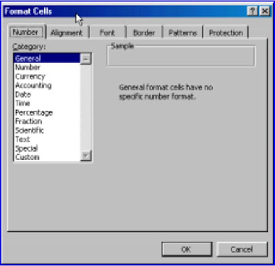
The menu command Format|Cells opens up the dialog box shown in Figure 6. From the Number tab one can set the format for numbers. The default setting is called General. You may wish to experiment with the Fixed and the Currency setting. If you click on the Fraction item you will see that it is possible to have fractional values displayed as quarters, eighths, etc.

Figure 6

The command Format|Column may be used to alter the width of a column. The default width is 8.38 units. A group of columns may be altered by selecting them in the column heading row before opening the Format|Column dialog. One of the most useful items on this dialog is the AutoFit Selection which makes the columns just the right width to hold their contents. If a column is given a width that is too small to hold a numeric value, the value will be displayed as ########. The solution is to (a) widen the cell and/or (b) display the value with fewer decimals if possible.

To experiment with formatting, make the worksheet shown in Figure 7. The vertical text was typed in normally and the cells were formatted with Format|Cells and opening the Alignment tab. The columns with this text were formatted for AutoFit. Using Tools|Options, and opening the View tab, the gridlines were removed from this worksheet.

Training completed
	Cash register	Customer inquiry	Inventory check
Damian	x	x
Jo		x	x
Justin		x
Nichola	x	x
Simon		x	x
Tim	x	x	x